Refer to Table 14-6. What Is the Total Revenue From Selling 4 Units?

Learning Objectives

• Determine profits and costs by comparison total revenue and total price
• Utilize marginal revenue and marginal costs to find the level of output that will maximize the house's profits

How Perfectly Competitive Firms Make Output Decisions

A perfectly competitive firm has only one major decision to make—namely, what quantity to produce. To understand why this is so, consider the bones definition of profit:

[latex]\brainstorm{array}{l}\text{Profit}=\text{Total revenue}-\text{Full cost}\hfill \\ \text{ }=\left(\text{Price}\right)\left(\text{Quantity produced}\correct)-\left(\text{Average cost}\correct)\left(\text{Quantity produced}\right)\hfill \end{array}[/latex]

Since a perfectly competitive house must accept the toll for its output equally adamant past the production'due south marketplace demand and supply, information technology cannot choose the price it charges. Rather, the perfectly competitive house tin choose to sell whatsoever quantity of output at exactly the same price. This implies that the house faces a perfectly elastic need curve for its product: buyers are willing to buy whatsoever number of units of output from the firm at the market price. When the perfectly competitive business firm chooses what quantity to produce, then this quantity—along with the prices prevailing in the market for output and inputs—will decide the firm'southward total revenue, total costs, and ultimately, level of profits.

Determining the Highest Profit by Comparing Total Revenue and Total Toll

A perfectly competitive firm can sell equally large a quantity as it wishes, as long equally it accepts the prevailing market toll. Total revenue is going to increase as the business firm sells more, depending on the cost of the product and the number of units sold. If you increase the number of units sold at a given price, then total revenue will increment. If the price of the product increases for every unit sold, and then total revenue too increases.

As an example of how a perfectly competitive firm decides what quantity to produce, consider the case of a small farmer who produces raspberries and sells them frozen for $4 per pack. Sales of one pack of raspberries will bring in $four, ii packs will exist $8, three packs will be $12, and and then on. If, for example, the price of frozen raspberries doubles to $viii per pack, then sales of one pack of raspberries volition exist $viii, ii packs will be $sixteen, three packs volition be $24, then on.

Total revenue and total costs for the raspberry farm are shown in Table 1 and as well appear in Figure ane.

Table 1. Total Acquirement, Total Cost, and Profit at the Raspberry Farm

Quantity (Q)	Total Revenue (TR)	Total Cost (TC)	Profit
0	$0	$62	−$62
10	$40	$xc	−$50
twenty	$eighty	$110	−$30
xxx	$120	$126	−$vi
40	$160	$138	$22
50	$200	$150	$l
60	$240	$165	$75
70	$280	$190	$90
fourscore	$320	$230	$90
90	$360	$296	$64
100	$400	$400	$0
110	$440	$550	$−110
120	$480	$715	$−235

In Figure 1, the horizontal centrality shows the quantity of frozen raspberries produced. The vertical axis shows both total acquirement and full costs, measured in dollars. The total cost curve intersects with the vertical axis at a value that shows the level of stock-still costs, and and then slopes upward, first at a decreasing rate, then at an increasing rate. In other words, the cost curves for a perfectly competitive firm have the same characteristics as the curves that nosotros covered in the previous module on production and costs.

Try Information technology

Effigy one. Total Acquirement, Total Cost and Profit at the Raspberry Subcontract. Total revenue for a perfectly competitive firm is an upward sloping directly line. The slope is equal to the price of the proficient. Total cost also slopes up, but with some curvature. At higher levels of output, total cost begins to slope upward more steeply because of diminishing marginal returns. Graphically, profit is the vertical altitude between the full revenue curve and the full price curve. This is shown as the smaller, down-curving line at the bottom of the graph. The maximum profit will occur at the quantity where the difference between full revenue and full cost is largest.

Based on its total revenue and full cost curves, a perfectly competitive firm like the raspberry subcontract can calculate the quantity of output that volition provide the highest level of profit. At whatsoever given quantity, total revenue minus total cost will equal profit. One way to determine the most profitable quantity to produce is to see at what quantity total revenue exceeds full price past the largest amount.

Effigy one shows full revenue, full cost and profit using the information from Tabular array 1. The vertical gap between total revenue and full cost is profit, for example, at Q = 60, TR = 240 and TC = 165. The difference is 75, which is the summit of the profit curve at that output level. The business firm doesn't make a profit at every level of output. In this case, total costs will exceed full revenues at output levels from 0 to approximately 30, and so over this range of output, the house will be making losses. At output levels from twoscore to 100, total revenues exceed total costs, and then the firm is earning profits. However, at any output greater than 100, total costs again exceed full revenues and the firm is making increasing losses. Total profits appear in the final column of Table ane. Maximum profit occurs at an output between 70 and 80, when profit equals $90.

Try It

A college price would mean that total revenue would be higher for every quantity sold. Graphically, the total acquirement curve would be steeper, reflecting the higher price as the steeper gradient. A lower price would flatten the total revenue curve, pregnant that total acquirement would exist lower for every quantity sold. What happens if the toll drops low plenty so that the total revenue line is completely below the total cost curve; that is, at every level of output, full costs are higher than total revenues? In this instance, the best the firm tin can do is to suffer losses. Notwithstanding, a turn a profit-maximizing firm will prefer the quantity of output where total revenues come closest to total costs and thus where the losses are smallest.

Comparing Marginal Revenue and Marginal Costs

The approach that we described in the previous section, using total revenue and total toll, is not the just arroyo to determining the profit maximizing level of output. In this department, nosotros provide an alternative approach which uses marginal acquirement and marginal cost.

Firms frequently do not have the necessary data they need to draw a consummate full cost curve for all levels of production. They cannot exist sure of what total costs would await like if they, say, doubled product or cut product in half, because they have not tried information technology. Instead, firms experiment. They produce a slightly greater or lower quantity and observe how it affects profits. In economic terms, this practical arroyo to maximizing profits means examining how changes in production affect marginal revenue and marginal toll.

As mentioned before, a firm in perfect competition faces a perfectly elastic demand curve for its product—that is, the firm's demand curve is a horizontal line drawn at the market price level. This likewise means that the business firm's marginal revenue bend is the same as the firm's demand curve. Every time a consumer demands ane more unit of measurement, the firm sells one more unit and acquirement increases by exactly the aforementioned amount equal to the market place price. In this example, every time the house sells a pack of frozen raspberries, the house'due south revenue increases by $4, as you tin see in Table ii. This condition only holds for price taking firms in perfect competition where:

[latex]\text{marginal revenue = price}[/latex]

The formula for marginal revenue is:

[latex]\text{marginal revenue = }\frac{\text{change in total revenue}}{\text{change in quantity}}[/latex]

Tabular array 2. Marginal Acquirement for Raspberries
Cost	Quantity	Total Acquirement	Marginal Acquirement
$four	1	$4	–
$4	ii	$eight	$4
$iv	iii	$12	$4
$4	4	$16	$four

Try Information technology

Notice that marginal revenue does not change as the business firm produces more output. That is considering the cost is determined by supply and demand and does not change as the farmer produces more (keeping in mind that, due to the relative small size of each firm, increasing their supply has no touch on on the full market supply where cost is adamant).

Effigy 2. Market Price. The equilibrium price of raspberries is determined through the interaction of market place supply and market place demand at $4.00.

Since a perfectly competitive firm is a price taker, it can sell whatever quantity it wishes at the market-determined toll. Marginal cost, the price per boosted unit sold, is calculated past dividing the change in total cost by the change in quantity. The formula for marginal cost is:

[latex]\text{marginal price = }\frac{\text{change in total cost}}{\text{change in quantity}}[/latex]

Different marginal acquirement, ordinarily, marginal cost changes as the business firm produces a greater quantity of output. At first, marginal cost decreases with additional output, simply so it increases with additional output. Once again, annotation this is the aforementioned every bit nosotros found in the module on production and costs.

Tabular array 3 presents the marginal acquirement and marginal costs based on the total revenue and total price amounts introduced earlier. The marginal revenue bend shows the additional revenue gained from selling 1 more than unit of measurement, as shown in Figure 3.

Table three. Marginal Revenues and Marginal Costs at the Raspberry Farm

Quantity	Total Acquirement	Marginal Acquirement	Total Cost	Marginal Cost	Profit
0	$0	$4	$62	–	-$62
10	$xl	$4	$90	$ii.80	-$fifty
20	$lxxx	$4	$110	$2.00	-$xxx
30	$120	$4	$126	$1.threescore	-$half dozen
40	$160	$4	$138	$1.20	$22
50	$200	$four	$150	$1.20	$l
lx	$240	$4	$165	$1.fifty	$75
70	$280	$4	$190	$ii.50	$90
80	$320	$4	$230	$4.00	$90
90	$360	$4	$296	$6.60	$64
100	$400	$4	$400	$x.40	$0
110	$440	$4	$550	$15.00	-$110
120	$480	$4	$715	$xvi.fifty	-$235

In the raspberry farm example, marginal cost at commencement declines as product increases from x to 20 to xxx packs of raspberries. But so marginal costs first to increment, due to diminishing marginal returns in production. If the business firm is producing at a quantity where MR > MC, similar xl or 50 packs of raspberries, so it tin increase profit by increasing output. The reason is since the marginal revenue exceeds the marginal toll, additional output is calculation more to profit than it is taking away. If the firm is producing at a quantity where MC > MR, like 90 or 100 packs, and then it can increment profit by reducing output. The firm's turn a profit-maximizing level of output will occur where MR = MC (or at a level close to that point).

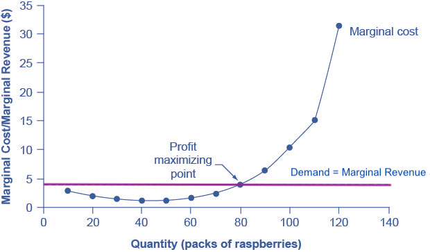
Figure 3. Marginal Revenues and Marginal Costs at the Raspberry Farm. For a perfectly competitive firm, the demand bend s a horizontal line equal to the market place price of the good, Since cost doesn't change with additional output, the need curve is also the marginal revenue (MR) bend. The marginal cost (MC) curve is sometimes initially downward-sloping, just is somewhen upwards-sloping at college levels of output as diminishing marginal returns kick in. The firm will maximize profit at the level of output where MR = MC. In the example of the raspberry subcontract, this occurs at 80 packs of strawberries.

In this example, the marginal revenue and marginal cost curves cross at a price of $4 and a quantity of 80 produced. If the farmer started out producing at a level of 60, and then experimented with increasing production to seventy, marginal revenues from the increment in product would exceed marginal costs—and so profits would rise. The farmer has an incentive to continue producing. At a level of output of fourscore, marginal price and marginal revenue are equal so profit doesn't change. If the farmer then experimented further with increasing production from 80 to 90, he would find that marginal costs from the increase in production are greater than marginal revenues, and so profits would decline.

The profit-maximizing choice for a perfectly competitive firm will occur at the level of output where marginal acquirement is equal to marginal cost—that is, where MR = MC. This occurs at Q = 80 in the figure.

Does Profit Maximization Occur at a Range of Output or a Specific Level of Output?

Table 1 showed that maximum turn a profit occurs at any output level between 70 and 80 units of output. But MR = MC occurs just at lxxx units of output. How can do we explain this slight discrepancy? As long as MR > MC. a profit-seeking firm should keep expanding production. Expanding production into the zone where MR < MC reduces economic profits. It's true that profit is the same at Q = lxx and Q = fourscore, but it's only when the firm goes across that that encounter that profits fall. Thus, MR = MC is the signal to terminate expanding, so that is the level of output they should target.

Because the marginal revenue received by a perfectly competitive business firm is equal to the price P, we tin also write the turn a profit-maximizing dominion for a perfectly competitive firm as a recommendation to produce at the quantity of output where P = MC.

Attempt It

Watch It

Watch this video to do finding the profit-maximizing signal in a perfectly competitive business firm. Mr. Clifford reminds us that in a perfectly competitive marketplace, the need bend is a horizontal line, which also happens to exist the marginal revenue. Y'all can use the acronym MR. DARP to remember that marginal revenue=need=average revenue=price. The platonic product bespeak is the place where MR=MC.

Try It

These questions allow y'all to get every bit much practise as yous need, every bit you lot can click the link at the top of the first question ("Try another version of these questions") to become a new prepare of questions. Practice until y'all feel comfy doing the questions.

Try It

These questions allow yous to get equally much do as you need, as you can click the link at the top of the first question ("Try another version of these questions") to go a new set of questions. Practice until you experience comfortable doing the questions.

Endeavor Information technology

These questions let yous to get as much do equally yous need, as you can click the link at the top of the first question ("Effort some other version of these questions") to become a new gear up of questions. Practice until yous feel comfortable doing the questions.

Glossary

marginal revenue:

the additional acquirement gained from selling one more unit of output

profit:

 the difference between full revenues and total costs

profit-maximizing rule for a perfectly competitive business firm:

produce the level of output where marginal revenue equals marginal cost

buttsoutte1975.blogspot.com

Source: https://courses.lumenlearning.com/wmopen-microeconomics/chapter/profit-maximization-in-a-perfectly-competitive-market/

Share this post